|
|
|

|
Site Index: In This Section:
|
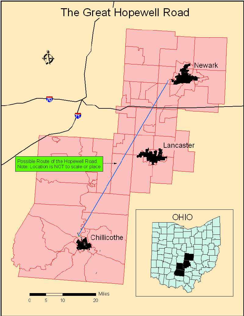
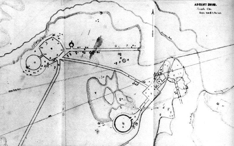
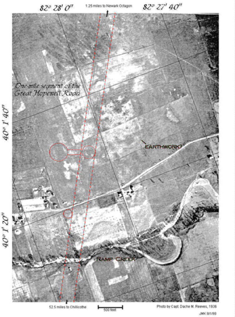
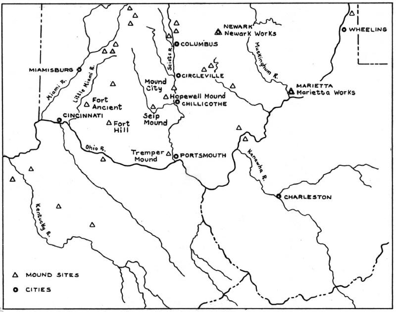
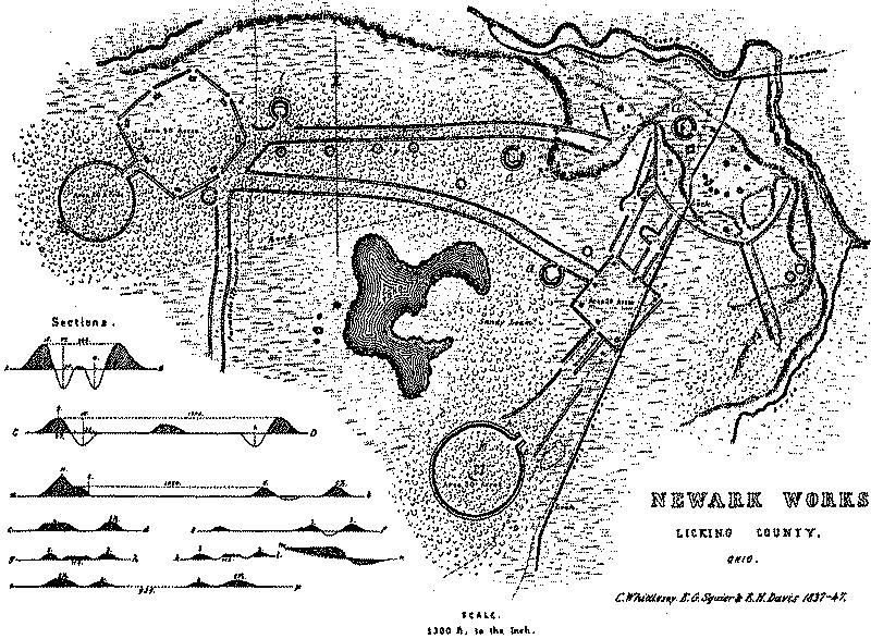
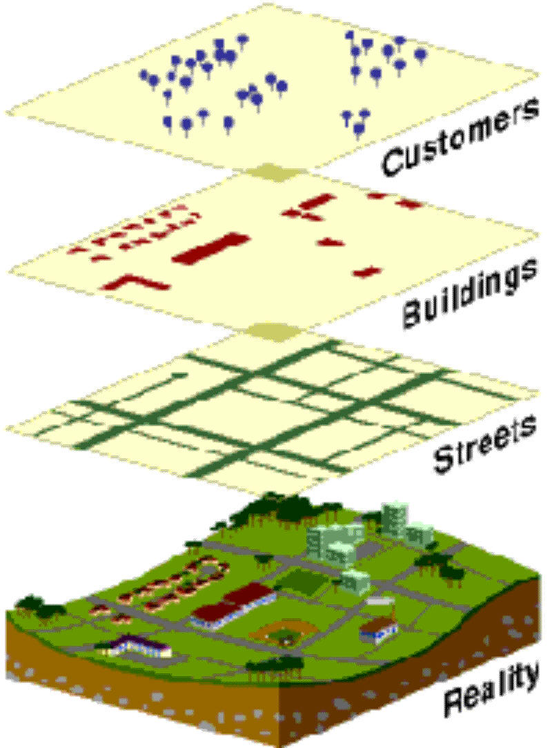
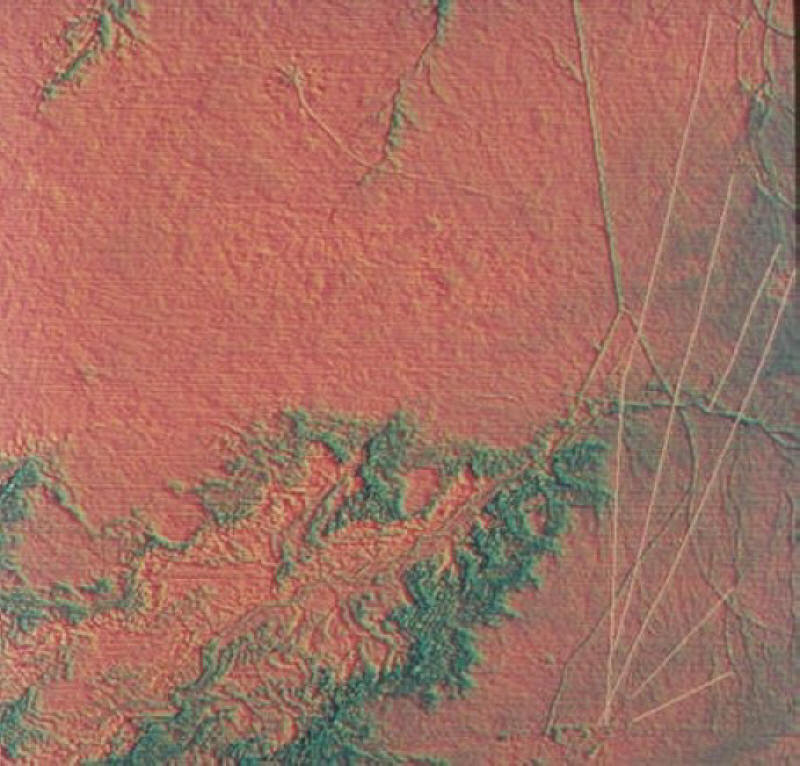
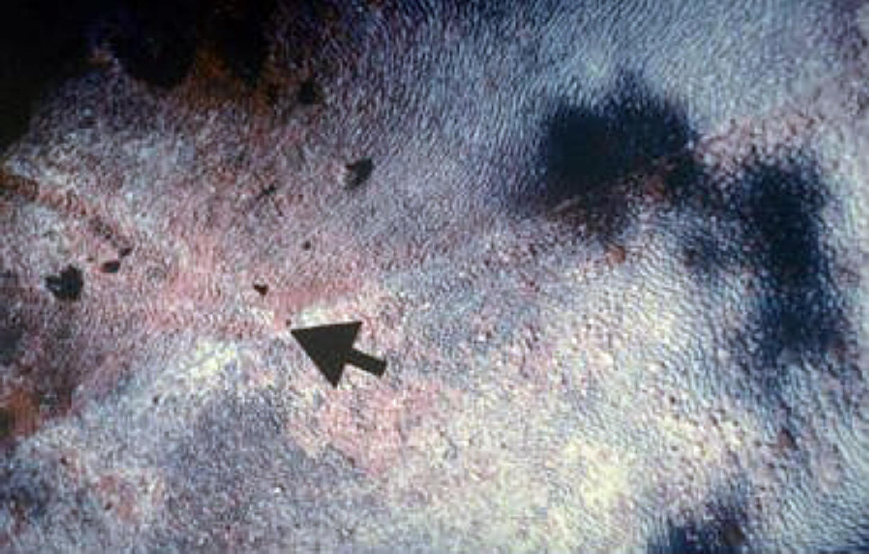
Hopewell RoadGIS Solutions Towards Pathway DiscoveryAcknowledgments The author wishes to give thanks to a few specific individuals without whom this project might never have been completed. First and foremost would be Dr. Brad Lepper, for without his initial prompting, the idea for this research would never have been come about in the first place. Following Brad is fellow cartographer and Ohio University alumnus Nicole Stump. Nicole helped with all too many glitches and was there for me to bounce ideas off of whenever I needed to focus and move forward. Next up would be my advisor for this project, Dr. James Lein. His knowledge of GIS, along with his confidence in me, aided me more than he can possibly know. And finally, there is my good friend Thomas Twitchell, whose editing skills are unparalleled. To each of you, as well as to the numerous others whom I have most likely forgotten, many thanks! Table of Contents 2. National Land Cover Classification System 1. Map of Projected Hopewell Road 2. 1862 Salisbury Map of Newark, Ohio Earthworks 5. Kavasch Adena Mounds Site Map 6. 1848 Squier & Davis Map of Newark, Ohio 8. NASA Chaco Canyon TIMS Image 9. NASA Costa Rica Color Infrared Photo 12. Study Area Suitability Map 13. Map of Routes Based on Suitability Models 14. Map of Route to Chillicothe Based on Cost 15. Map of Route to Lepper’s Southernmost Location 16. Map of Ohio Historical Society Mounds Chapter 1 In the southwestern United States, the Anasazi built their own system of sacred pathways replicating a spiritual landscape described in their origin myths. Until recently, such roads were unknown in eastern North America, though nineteenth-century observers had recorded short stretches of parallel earthen walls leading to and from the large geometric enclosures of the Hopewell, a people who thrived in the valleys of what is now southern Ohio from ca. 100 B.C. to ca. A.D. 400. Dr. Bradley T. Lepper, 1994 If people said that a prehistoric road defined by earthen walls existed in Ohio, they might dismissed as having overactive imaginations. Moreover, if they said that this road stretched between the present-day cities of Newark and Chillicothe, Ohio, a distance of some 60 miles (Figure 1), they might be dismissed completely. However, in the end, they might agree with them, for evidence exists that would suggest the plausibility of just such a road. Traversing hills, valleys, and streams, the Great Hopewell Road might have begun at the earthworks located in Newark, Ohio and ended near Chillicothe, at the site of another ancient earthwork named the High Bank Works due of its location on the bank of a tributary of the Scioto River. It is tempting to try to connect these two earthworks for they both contain circular and octagonal arrangements. High Bank Works has an earthen circle that is approximately the same size as the Newark circle, and it is aligned at 90 degrees to the axis of the Newark Earthworks, suggesting that one of the complexes might have been built to complement the other, perhaps through a unifying religious ritual that followed the 18.6-year lunar cycle (Aveni 2000:226, Lepper 1995). More important, the Scioto Valley was the “undisputed center of Ohio Hopewell culture” (Lepper 2002), so a road passing through the region could have linked the area together. But why would there have been such a grandiose road linking these two monumental works, and how can one go about proving it actually existed? That such a Great Road existed seems to be more in the realm of probability than possibility. Aveni (2000) and Nials et al, (1987) examine how other studies have shown prehistoric cultures engaged in very similar road-building phenomena. In the Yucatan, for example, Mayan roads connecting various ceremonial and sacred sites are well known. Similarly, the Anasazi of the southwestern United States constructed sacred roads and pathways between their most important places of pilgrimage. The same can be said of numerous places in Europe, India, and China. These passageways have been referred to as ley lines (Aveni 2000), shaman trails, fairy paths, or even spirit paths. Often, however, these roads are so antediluvian, and the sites they once connected have been so altered by succeeding cultures, that they are difficult, if not impossible, to detect. The Hopewell Indians were a well-traveled people with deep-rooted religious beliefs. Additionally, they were “wide ranging in their contacts, with a resource network that reached for hundreds of miles in all directions” (Romain 2000:2). Proving that a Great Hopewell Road exists would have a special meaning to Western archaeologists for it would be both pre-Anasazi and pre-Mayan in conception and would be the first discovered in the eastern United States. Much of the direct confirmation for the existence of just such a road comes in the form of early land surveys, aerial photographs, and, for some, just a plain “gut” feeling about the road’s existence. Caleb Atwater, one of Ohio's first archaeologists, suggested in 1820 that the parallel walls that ran southwest from Newark's octagon might extend 30 miles or more. In 1862, James and Charles Salisbury, early residents of Newark, traced these same walls. Although they did not follow the road to its end, the Salisburys noted that “These works have been accurately surveyed and described – on account of the discovery of outside walls, connected with the fortified ways & other Earthworks of interest. One of the highways has been traced over six miles in the direction of Circleville. These walls are all of clay – differing materially from the soil on which they repose – which appears to indicate that originally they may have been constructed of adobe; or sun dried brick; similar to the fortified highways of the Incas of Peru” (Salisbury and Salisbury. 1862). One of the most important pieces of evidence, however, is the map (Figure 2) that the Salisburys drew in 1862. Their map depicts the Newark Earthworks and shows a series of parallel walls appearing to connect the various enclosures there. This diagram was misplaced for decades following the Civil War, only to be rediscovered by Dr. Brad Lepper in 1991 at the American Antiquarian Society in Worcester, Massachusetts. The Salisburys’ map reinforces maps drawn by Squier and Davis in 1848, and Wyrick in 1866, while at the same time expanding on their work by giving details not previously mentioned. Other evidence comes in the form of aerial photography taken in the early 1930s, as well as more recently. For example, Capt. Dache M. Reeves of the U.S. Army Air Corps worked with the Ohio State Archaeological and Historical Society in an aerial survey of various prehistoric earthworks and in 1936 published a preliminary article entitled A Newly Discovered Extension of the Newark Works. Reeves’ photographs (Figure 3) show lines and circles on the earth that could be the route of a possible Hopewellian Road, along with other mounds located nearby. Reeves’ reconnaissance seems to confirm that such a road was in all likelihood a reality. Lepper, of the Ohio Historical Society, has recently searched along this same corridor for traces of road using aerial reconnaissance and archival photography (both conventional and infrared) and has identified traces of parallel lineation along the projected route in several places (Figure 4). Specifically, Lepper contends that the first, and most convincing, segment can be found 26 kilometers south of Newark, while another is located at the projected terminus of the Great Hopewell Road near Chillicothe. The question yet remains: Did the ancient Hopewell Indians build a direct roadway between the Newark Earthworks and the earthworks near Chillicothe? Now more than ever, historical research is interdisciplinary. In the past 100 years, destructive forces have nearly obliterated what remains of the Hopewell earthworks in Ohio. Whether plowed under, bulldozed down, or paved over, most Hopewell artifacts, along with the culture they represent, seem to have eluded preservation. Still though, it is reasonable to say that a wealth of information on Hopewell culture awaits discovery. It is my contention that with the combined use of remote sensing techniques and traditional archaeological methods the Great Hopewell Road will once more appear. More specifically, the research conducted in this thesis will examine the roles that slope, land cover, proximity to water, etc., would have played in the Hopewell’s decision of where to locate just such a road? Chapter 2 In the Ohio Valley we have found places of contact and mixture of two races, and have made out much of interest, telling of conflict and defeat, of the conquered and the conquerors. … Our explorations have brought to light considerable evidence to show that … a race of men, with short, broad heads, reached the valley from the southwest. Here they cultivated the land, raised crops of corn and vegetables, and became skilled artisans in stone and their native metals, in shell and terra-cotta, making weapons and ornaments and utensils of various kinds. Here were their places of worship. Here were their towns, often surrounded by earth embankments, their fixed places for burning their dead, their altars of clay, where cremation offerings, ornaments, by the thousands were thrown upon the fire. Upon the hills near by were their places of refuge or fortified towns…” Frederic W. Putnam, 1888 Ancient Indian tribes have long been noted on the American frontier, dating back more than 4,000 years. Indeed, the Spaniard Hernando De Soto (1500? – 1542) met the Natchez on his voyages exploring the Americas in 1540, noting that they built large earthen mounds using just the strength of their tribes people. Garcilaso de la Vega, one of the chroniclers of De Soto’s expeditions to the Americas, recorded that leading up to the houses that stood atop the mounds, “the Indians build two, three, or more streets, according to the number that are necessary, straight up the side of the hill. These streets are fifteen or twenty feet in width and are bordered with walls constructed of thick pieces of wood…” (Silverberg 1986:19). Two hundred years later, European trappers and settlers would begin moving west past the Allegheny Mountains into the Ohio River Valley. It would be there that they would have their first encounters with the legacies of the prehistoric Indian tribes – strange earthen forms dotting the land. Some of these mounds were conical, others flat-topped. Some even took the appearance of humans or animals. The size of these structures astonished the settlers. One great mound, in Ross County, Ohio, was shown to have been made of thousands of loads of earth. Indeed, Ross County alone proved to have 500 mounds and some 100 enclosures (Silverberg 1986:13). Yet these mysterious and wondrous mounds left behind no obvious clues as to who built them! Indeed, not even the natives who were present when the settlers arrived could answer questions about them, thereby forming the basis of a “lost race” that had simply vanished. Thus, shortly after coming across these unique structures, early scholars set out to map, study, and excavate them in an effort to learn what they could of the ancient people who inhabited the lands before them. Some of the mounds contained human bones; others held unusual artifacts made of copper or shells; yet others contained nothing at all. Research has concluded that the first major mound builders were the Adena Indians, so named after the 1901 excavation of a mound located on the Adena estate of former Ohio governor Thomas Worthington, west of Chillicothe. A tall, robust people who “shared a profound sense of nature and appreciation of life, each other and death” (Kavasch 2004:53), the Adena were both hunters and farmers living throughout the Ohio River Valley. Also well known for their ability to make finely crafted pipes, the Adena developed extensive trade routes, with each village supplying its own unique objects to trade. By about 500 B.C., the Adena were prospering and their villages growing. (Kavasch 2004:55)They began to construct mound-building centers, with the largest of these within a 150-mile radius of Chillicothe (Figure 5). At some point, they began the practice of placing their honored dead in large conical-shaped mounds, around which were built earthen ridges. Caleb Atwater, an early Ohio historian, was particularly impressed by the geometric regularity of the main Circleville enclosures – circles and squares constructed with such accuracy that they seemed to indicate that the builders had been master surveyors. “Atwater correctly saw that such elaborate earthworks must have been the products of a dense population well supplied with food. A sparse tribe of huntsmen, preoccupied with the need simply to keep alive, could never have built them” (Silverberg 1986:59). Years after Atwater’s revered 1820 essay, Description of the Antiquities Discovered in the State of Ohio and Other Western States, was published, the American Ethnological Society began a search for someone to undertake new research on the American Indians. They found their man in Ephraim George Squier, a newspaper editor and part-time politician (Silverberg 1986:82). Squier joined with Dr. E.H. Davis, a Chillicothe physician, and together they excavated numerous sites, culminating in their masterpiece work, Ancient Monuments of the Mississippi Valley. With many attractive maps and surveys (Figure 6), the duo seemed to enjoy describing the enclosures and walled avenues of southern Ohio, and they, like Atwater, were awed by the precision of the earthworks. In the early 1880s, it became apparent that the mounds might soon disappear forever, taking with them a wealth of as yet undiscovered information. Congress approved $5,000 for a full-scale scientific investigation and, in 1888, Fredrick W. Putnam, curator of Harvard’s Peabody Museum, advanced the theory that instead of a single race of mound builders in the Ohio Valley, there was a succession of races. He was the first to offer this idea, now widely accepted. In 1894, Cyrus Thomas, a Smithsonian scientist, published his report chasing away the notion that the mound builders were a “lost race”. It soon became clear that the skulls exhumed from the mounds came from not one, but from many differing tribes of prehistoric Indian people who shared many similarities over time. Archaeologists now believe that around 400 B.C. a new group of people began to enter the territory of the Adena. (Silverberg 1986:179). The newcomers belonged to the Hopewell culture, named for a 110-acre site in Ross County, Ohio, where their traits were first observed. The Hopewell adopted the basic patterns of Adena life, but expanded upon them, thereby making them their own. They were the true “mound builders” whom nineteenth century writers made so much of; they were the makers of the vast quantities of burial mounds, as well as the celebrated earthen embankments that covered hundreds of acres. Still though, the question of the relationship between the two cultures remains unsettled. Most archaeologists believe “that Adena was earlier than Hopewell; that Hopewell represented a stock of long-headed intruders who came into the territory controlled by the round-headed Adena folk; that the burial and earthwork customs of Hopewell were borrowed from Adena; that there was close contact and even intermarriage between Adena and Hopewell; and that all Adena sites had been abandoned before the greatest years of the Hopewell Culture” (Silverberg 1986:199). Don W. Dragoo of Pittsburgh’s Carnegie Museum, as recounted by Silverberg (1986), doubts many of the earlier theories regarding how the Adena and Hopewell cultures arose. Rejecting the belief that Hopewell ideas were drawn from the Adena, he instead believes that the Hopewell and Adena may have developed side by side. Many archaeologists are coming to accept just such an argument, seeing it as a more plausible concept (Silverberg 1986). Whether or not their practices arose independently of the Adena, the Hopewell shared certain economic, political, and spiritual beliefs with them. Hopewell traits were found to varying degrees in the Middle Woodland groups that lived from present-day Missouri to New York State, with the largest concentration in what is now Ohio. The Hopewell culture flourished in central and southern Ohio between approximately 200 B.C. and A.D. 500. Their time was characterized by the construction of large geometric earthworks with associated mounds and parallel embankments. While the Hopewell left no known written records, they did leave a legacy of mystery. Silverberg explains various archaeological definitions, stating that “A culture is a specific social group with a distinct way of life. A tradition is a broadly defined way of life, practiced in more or less the same manner by different cultures at different times. A period is a certain span of time during which a particular tradition is dominant. In Ohio, where the Woodland Tradition was the main way of life from about 1000 B.C. to A.D. 700, the term Burial Mound Period has been assigned to those centuries” (Silverberg 1986:171). Like the Adena culture, the Hopewell buried their dead in large mounds along with finely crafted pieces meant to accompany them into the afterlife. These objects were made from mica, copper, obsidian, silver, and other exotic materials brought to Ohio from as far away as the Atlantic, the Gulf of Mexico, and what is now the western United States (Kavasch 2004:86). The Hopewell and the Adena traded amongst themselves and with other native tribes. They shared common religious practices and beliefs. Yet unlike the Adena, the Hopewell had a strict class system with a separation of labor within the community (Kavasch 2004: 105). Abundant natural resources allowed the Hopewell to develop a cohesive society able. This enabled them to make the significant investment in time and labor necessary to construct mounds and earthworks, develop finely crafted objects, bury their dead in a grandiose style, and maintain long-distance contact with other prehistoric societies. While individual territories were most likely controlled by a local chief, the communities would gather together for festivals, religious ceremonies, or trading (Kavasch 2004: 63). Living near the incredible earthworks they built, the Hopewell might have traveled The Great Hopewell Road as a way to communicate, proceed on religious precessions or quests, or simply attend the activities of another community. “At present, we can give no firm answer to the question of Hopewell origins. It now seems that the Hopewell emerged from the obscurity of the woodlands, borrowed some ideas from the Adena, some from distant Mexico, thought up some themselves, and drew them all together to create a dazzling, wealthy society that flourished for centuries, indulged in splendid burial customs unknown elsewhere in the prehistoric United States, imposed its way of life on an area covering thousands of square miles, sent traders to the shores of far-off seas, amassed great treasure to thrust into earthen mounds, erected phenomenal structures in geometrical patterns – and faded away, leaving behind the ramparts and mounds that aroused such wonder in our great-grandfathers” (Silverberg 1986:226). Today, the majority of the monuments built by the Hopewell, including the long parallel earthen-walled avenues that so impressed Atwater and Squier, have vanished. The remaining earthworks stand as a testament to the Hopewell’s marvelous achievements. The Great Hopewell Road may have just been another one. Chapter 3 Archaeologists have always been intrigued by new analytical directions coupled with technical means, be they stratigraphy, seriation, radiocarbon dating, remote sensing, and now GIS, as avenues to hopefully, rather automatically, understand the “past” using contemporary data. James I. Ebert, 2000 Many of the world's archaeological and cultural treasures, such as the Egyptian pyramids and Britain's Stonehenge, are slowly falling victim to the ravages of pollution and the elements. But what of those treasures that have not been found yet? No doubt, many important archaeological sites lie beneath the soil, hidden from view. Some of these sites likely have been damaged by agriculture, mining, and other forms of human activity. Still others are probably imperiled. It falls upon geographers and archaeologists to try to detect, document, and map these sites before they are lost forever, leaving irreversible holes in our archaeological and cultural landscapes. Fortunately, the tools used to accomplish such a task are steadily advancing. Since the days of Heinrich Schliemann's search for ancient Troy, archaeologists have been confronted with the problem of how to record the spatial characteristics of archaeological or cultural data and, once recorded, how to analyze those data. This spatial information has historically been recorded on paper maps with varying accuracy and scales. When researchers wanted to perform analyses of these data, they were required to spend hours, if not days, transposing the information to new paper maps while making arduous measurements by hand. This time-consuming process is nearing its end as researchers move to take advantage of Geographic Information Systems for spatial analysis. Simply put, a Geographic Information System (GIS) combines layers of information about a place to give a better understanding of that place. However, in the strictest sense, a GIS is a computer system capable of assembling, storing, manipulating, and displaying geographically referenced information, and is designed to work with data referenced by spatial or geographic coordinates. In other words, a GIS is both a database system with specific capabilities for spatially referenced data, and a set of operations for working with and analyzing that data. A GIS is best thought of as a dynamic database for spatial data. It is a tool that can help researchers integrate a variety of data sources and types, as well as manage inventories, visualize data using dynamic maps, make decisions about resource management, and even perform modeling and analysis. Indeed, the power of GIS comes from its ability to link objects on a map to a database through the use of a query function. What layers (Figure 7) of information are combined depends on the purpose — finding the best location for a new store, analyzing environmental damage, or attempting to retrace ancient archaeological sites. GIS, which can use information from many different sources and in many different forms, can help with such analyses. The primary requirement for the source data is that the locations of the variables are known. Locations may be annotated by x, y, and z coordinates of longitude, latitude, and elevation, or by such systems as ZIP codes or highway mile markers. Any variable that can be located spatially can be fed into a GIS. Once a GIS layer is built, spatial relationships between mapped features can be analyzed for patterns that would not otherwise be readily apparent. Researchers can either analyze geographic data within a single layer or examine the relationships between multiple layers. Perhaps more important, such analyses can be conducted at almost any scale, from site specific to regional or even global. GIS is, therefore, a very powerful tool that can be used to conduct a variety of quantitative analyses, even when the researcher cannot get to the site in person. For the archaeologist attempting to uncover spatial relationships about the past, GIS has opened a door to the field not opened since the introduction of radiocarbon dating in the 1950s. What may become the most useful for this field is the application of predictive modeling. “Predictive models are tools for projecting known patterns or relationships into unknown times and places” (Westcott and Brandon 2000:6). In recent years, GIS has experienced explosive growth, and archaeology has been just one of the many disciplines that have been caught up in this technological whirlwind. Occurring over the past 10 to 15 years, this explosion reflects the importance of space, spatial concepts, and spatial modeling – both in the present day as well as in days gone by. Geographic variables exert a strong influence on human behavior today, and archaeologists are aware of the significance of this influence in the past. Geography also influences the degree of exposure of archaeological sites, and the degradation they face from human activity and natural forces. Management and research decisions are based on geography. Geographic analysis and modeling provide answers to a variety of questions, and they help those in charge make informed decisions about the areas under study. The continued improvement of GIS software is just one of the ways technology has changed the face of archaeology. The development of imaging systems with extraordinarily high spatial resolution and the introduction of ever more powerful personal computers have also played crucial roles. But policy changes have been important, as well. The U.S. government only recently (in 2000) began offering the civilian sector widespread use of Global Positioning Satellite technology, making it possible to locate sites with a high level of accuracy. Governments have also made accessible once-classified satellite images. Archaeologists have been quick to take advantage of these improvements and have been keenly interested in how these technologies can be effectively integrated (Aldenderfer 1986). For example, many projects now use satellite imagery to generate data about slope, land use, or vegetation cover of a survey area. Such imagery is also used routinely to build digital elevation models (DEMs) of project areas that, in combination with data derived from archaeological surveys, can be used to evaluate ancient trade routes or patterns in location preferences, as well as make numerous other assessments (Aldenderfer 1986.). DEMs are also used to create “viewsheds,” a key component of visualizing just how an ancient site might have appeared. Archaeologists are interested in finding out how ancient people may have successfully adapted to their environment and what factors may have led to their collapse or disappearance. For example, “Did they overextend the capacity of their landscape, causing destructive environmental effects which led to their demise? Can this information be applied to modern day societies so that such mistakes are not repeated?” New technologies such as GIS and remote sensing can be used as methodological procedures “for detecting, inventorying, and prioritizing surface and shallow-depth archaeological information in a rapid, accurate, and quantified manner. … Understanding how ancient man successfully managed [his resources] is important for the success of current and future societies” ( Sheets and McKee, 1988). Much of human history can be traced through the impacts of human actions upon the environment; the use of GIS and remote sensing technologies offer the archaeologist the opportunity to detect these impacts -- impacts that are often invisible to the naked eye. This information can then be used to address issues in human settlement, environmental interaction, and climate change. One of the foremost applications to make its way into the mainstream of archaeology was the use of aerial photography as a way to conduct surveys. Surprisingly, this technique owes its beginnings to the fierce combat of World War I. During the war, pilots noticed strange circles and squares from the air that were not visible on the ground, patterns that were not part of the modern landscape. Returning to these locations after the war, they discovered that these strange patterns were actually archaeological sites, ancient roads, or other features of buried landscapes. The earliest pioneers of “aerial archaeology” conducted their first surveys in Europe and the Middle East in the 1920s (Madry n.d.). Charles Lindbergh conducted similar surveys in the western United States in 1929 (Chaco Canyon) and Central America in the 1930s. The photographs he took of Chaco Canyon revealed an ancient roadway system whose extent could no longer be seen from the ground nor easily recognized from the air. In 1971, the old Lindbergh photographs were re-examined and the roadways were essentially rediscovered. This initiated a number of projects with the involvement of the Bureau of Land Management (BLM), the National Park Service (NPS), and the State of New Mexico’s Historic Preservation Office (SHPO). In 1982, a NASA project team attempted to locate the roadways and to trace them using Thermal Infrared Multispectral Scanner (TIMS) imagery from satellites (Figure 8). Possible sites often emit “signatures” of energy – fingerprints of a sort – and computers can be programmed to search for them in areas where actual land surveys have not yet been done (Arnold n.d.). The road system was detected through emissions of infrared radiation at a wavelength different from that of the surrounding vegetation. The project proved extremely successful, revealing roads that appear to have been 30 feet wide leading across the desert for great distances (Trombold 1991:7). Chaco Canyon also helped establish the value of remote sensing as a discovery tool. Such technology was also used in Costa Rica, where a team of professionals from NASA and the University of Colorado searched the mountains for traces of ancient footpaths (Figure 9). The footpaths proved to be the oldest known in the New World, buried under volcanic deposits and obscured from the air by a 150-foot jungle canopy. The difference in moisture level of the soils detected by TIMS led to their discovery. Although researchers saw no physical evidence of the footpaths on the ground, the team dug trenches to confirm their existence through archaeological investigation. In addition, by following the footpaths and using predictive modeling, the project team located approximately 60 settlements and other sites in areas of the Costa Rican mountains that had been believed to be uninhabited in prehistoric times (Sheets 1994). Aerial and satellite imagery can be particularly useful in identifying soil contexts and environmental indicators that may suggest the presence of archaeological sites. Otherwise invisible aspects of the prehistoric or historic natural environment and such early human modifications of the land as roads, trails, fields, and irrigation systems can be revealed with these techniques. While picks, shovels, and mesh screens are still classic tools of archaeology, high-tech tools such as global positioning systems and remote sensing instruments are becoming ever more prevalent. Finding things that reveal the past is the first crucial step in reconstructing it; remote sensing techniques can prove invaluable in site location modeling, giving researchers the ability to determine where historic sites of a given period may be located. While GIS has increasingly become a routine tool in parts of the commercial and administrative arena, much academic work is still aimed at exploring the possibilities of the technology. Within the research community, many computer-literate archaeologists have applied GIS to their field of interest, be it environmental archaeology, regional settlement studies or intra-site spatial analysis, as a logical extension to the use of special-purpose mapping or spatial analysis programs. A few have made it their special domain and explored the theoretical and methodological implications of this new technological integration. The result is that GIS is being used on a daily basis by many archaeologists (Allen 1990). Chapter 4 There are a variety of ways in which a prehistoric road may be located, identified, and verified. These include remote methods such as aerial reconnaissance, interpretation of aerial photography; and ground methods such as examination of surface physical characteristics (width, depth, border elements, constructed features), distribution of road-associated structures (Bonito Phase great houses, herraduras, zambullidas) and subsurface physical characteristics (modified soil structure, consistence, color).” Fred Nials et al, 1987 GIS has been shown to be a valuable tool in the discovery of long-lost archaeological sites. It has been used to locate prehistoric cities, routes of travel, and even the distribution patterns of pottery shards. Although GIS has been used by archaeologists in the past, the question remains: Can GIS be used to assist in the detection of the Great Hopewell Road? More specifically, what roles would slope, land cover, proximity to water, and proximity to other earthworks have played in the Hopewell’s decision of where to locate such a road? In order to solve such a spatial problem, the steps that need to be performed must be thoroughly thought out. To that end, three components were outlined: data collection, data preparation, and analysis and modeling. Data Collection Much of the data used in this model came from online repositories. These included the U.S. Geological Survey (USGS) EROS Data Center, the State of Ohio’s Geographically Referenced Information Program (OGRIP), and the GISDataDepot. In addition, the cooperation of Brent Eberhard from the Ohio Historical Society was enlisted so that database information pertaining to known places of prehistoric Indian activity could be obtained. Specifically, Eberhard was asked to put together a query on the Ohio Archaeological Inventory with the following parameters: 1. Ross, Fairfield, Pickaway, and Licking Counties 2. Sites that match any of the following criteria: · village · hamlet · habitation i. included because they must have high densities of a considerable variety of artifact types - "near villages" or "pre-villages/hamlets" · all mound types · prehistoric cemeteries · burials · prehistoric petroglyphs Additionally, Dr. Brad Lepper was directly involved with this project and provided exact coordinates for suspected locations within the study area. Photographs, as well as GPS readings, were later taken from these sites. Perhaps most important for this study, however, was the use of DEM information, which was acquired from the USGS National Elevation Dataset (NED). The NED is a seamless mosaic of best-available elevation data. The majority of the dataset was published in 1999, but some of it was updated in August 2001. It was the most recent edition available when this project was started. Bounding coordinates of latitude and longitude used for the study area were as follows: · West Bounding Coordinate: -83.08485 · East Bounding Coordinate: -82.3319736 · North Bounding Coordinate: 40.122814 · South Bounding Coordinate: 39.282714 These coordinates resulted in the following 49 quad maps, all with a spatial resolution of 30 meters, being supplied by the USGS and used for data extraction:
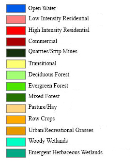
Additionally, an Ohio land cover dataset was obtained from the USGS using the same bounding coordinates and spatial resolution as above. The National Land Cover Dataset (NLCD) was compiled from Landsat satellite TM imagery (circa 1992), with the Ohio portion of the NLCD created as part of land cover mapping activities for Federal Region V, which includes Illinois, Indiana, Michigan, Minnesota, Ohio, and Wisconsin.
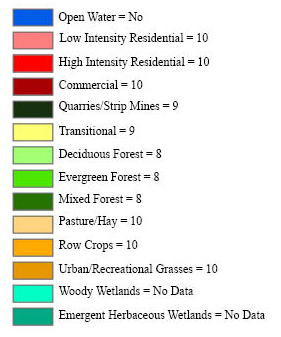
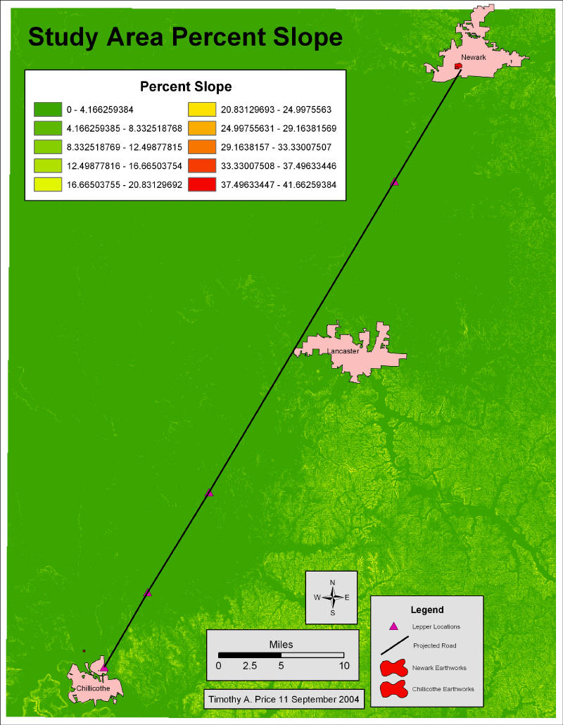
Data Preparation ESRI’s ArcGIS software package, version 8.3, was utilized for the following procedures. 1. Because data collected from online repositories are not, as yet, of a uniform nature when it comes to coordinate systems used (UTMs, feet, longitude or latitude, for example) they were converted to the following standard coordinate system using the ArcToolbox conversion tool: NAD 1983 State Plane Ohio South FIPS 3402 Feet Lambert Conformal Conic False Easting: 1968500.000000 False Northing: 0.000000 Central Meridian: -82.500000 Standard Parallel 1: 38.733333 Standard Parallel 2: 40.033333 Latitude Of Origin: 38.000000 GCS North American 1983 2. As is the case with modern roads, it likely would have been preferable to build the Hopewell road on relatively flat ground. Therefore, a slope calculation was compiled using the digital elevation model previously downloaded from The National Map Seamless Data Distribution System, as noted above. Both percent and degree slope calculations were made using the DEM raster grid (new_dem). The percent slope map produced a more visually understandable map and was used throughout the rest of this model. · Degree Slope ranged from 0.00 to 22.62 degrees · Percent Slope ranged from 0.00 to 41.66 percent The slope layer (Figure 10) was then divided into 10 equal intervals and reclassified (step3) so that higher slopes had lower values, while lower slopes had higher values. Thus, a slope of 41.66% was given a value of 1. It was decided that certain land covers would have been better suited for road construction than others, taking into consideration the effort involved in moving across different land cover types. The land cover raster (new_landcover) previously downloaded from the USGS Seamless Web site was originally classified into 14 categories, as follows:
3. Deciding what land use was suitable in prehistoric times is an extremely arbitrary decision. For example, trees could have been cut down to build canoes or make fires, and farming, though done, was not as intensive as it is today. Therefore, the land use grid (new_landcover) was reclassified (step_5) into 3 broad categories and assigned the following values:
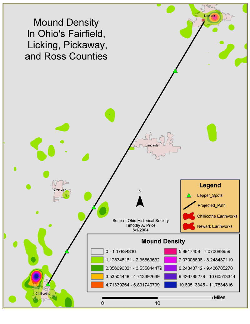
4. The road would have most likely been located near other ancient locations. The original Ohio Historical Society database had several locations listed without any coordinates given; these locations were deleted from the file to avoid conflicts. Additionally, the locations were first given in the form of UTM coordinates, which were then imported into ArcMap by using the “Add XY Data Wizard”. This file (corrected_mounds.dbf) was then converted into a shapefile and clipped (Clip_OHS_Mounds) so that only mounds within the study area were taken into account; there were originally 344 such sites listed in the database, but only 241 were located in the actual study area. The database was then converted into an ESRI raster (ohs_mounds) grid using the same coordinate system as mentioned above. This grid was classified so that cells had a value of 1 if a location was present and a value of 0 if one was not. 5. A density calculation was performed so that mound concentrations could be readily visualized. A kernel calculation was decided upon over a simple calculation as the result is a smoother distribution of values. Kernel density calculations work the same as simple density calculations, except that the points lying near the center of a raster cell's search area are weighted more heavily than those lying near the edge. A search radius of 10,000 feet was specified – again, an arbitrary number that best shows mound concentrations within the study area. Mound densities ranged from 0.2 to 2.1 mounds per square mile as shown in Figure 11). Next a straight line distance was calculated next using the ohs_mounds raster file giving a distance in feet. Straight Line Distance gives the distance from each cell in the raster to the closest source, in this case the prehistoric locations as given in the list supplied by the Ohio Historical Society. This new dataset, distan_to_OHS, was then reclassified (step8) into equal intervals. Values of 10 were given to areas closest to locations (the most suitable), while values of 1 were given to areas farthest from locations (the least suitable). Areas in between were ranked. 6. The road would have been located near rivers, so shapefiles were downloaded from Geocomm.com. Next, all of the files were merged and clipped so that only the study area was considered. This file was then converted into a raster file (merged_rivers). Following this, a straight line distance (dist_rivers) was calculated giving a distance in feet. This new dataset, dist_rivers, was then reclassified (reclas_rivers) into equal intervals. Values of 10 were assigned to areas closest to rivers (the most suitable), while values of 1 were assigned to areas farthest from rivers (the least suitable). Areas in between were ranked. 7. The road would have most likely been located near standing water bodies, so these shapefiles were also downloaded from Geocomm.com, merged, clipped into the study area, and converted into a raster file (merged_water). A straight line distance for this was calculated as well, giving a distance in feet. This new dataset, dist_water, was then reclassified (reclass_water) into equal intervals. Values of 10 were assigned to areas closest to the water (the most suitable), while values of 1 were assigned to areas farthest from the water (the least suitable). Areas in between were ranked. 8. The road would have been located near the earthworks in Chillicothe and Newark since it is assumed that the road would have linked those locations. The two major earthwork groups were digitized into two individual shapefiles (Newark_Earthworks and Chillicothe_Mounds) from digital air photos obtained from the State of Ohio’s OGRIP (Ohio Geographically Referenced Information Program) Web site. These shapefiles were then merged and converted into a raster grid (earthworks) where a value of 1 meant the presence of an earthwork. 9. A straight line distance was calculated giving a distance in feet to these two locations. This new dataset, step12_dist, was then reclassified (step12_reclas) into equal intervals. Values of 10 were assigned to areas closest to the earthworks (the most suitable), while values of 1 were assigned to areas farthest from the earthworks (the least suitable). Areas in between were ranked. Analysis and Modeling Because so many variables were initially chosen for this study, it became necessary to produce a suitability model as the first step. This type of model allows researchers to find areas that are the most suitable for particular objectives. In this model, datasets of slope, land cover, standing water bodies, rivers, earthworks, and prehistoric mound locations were examined. An arbitrary weighting scheme was chosen for the different datasets. Using the raster calculator function once again, the various datasets created previously were combined according to the percent of importance listed below:
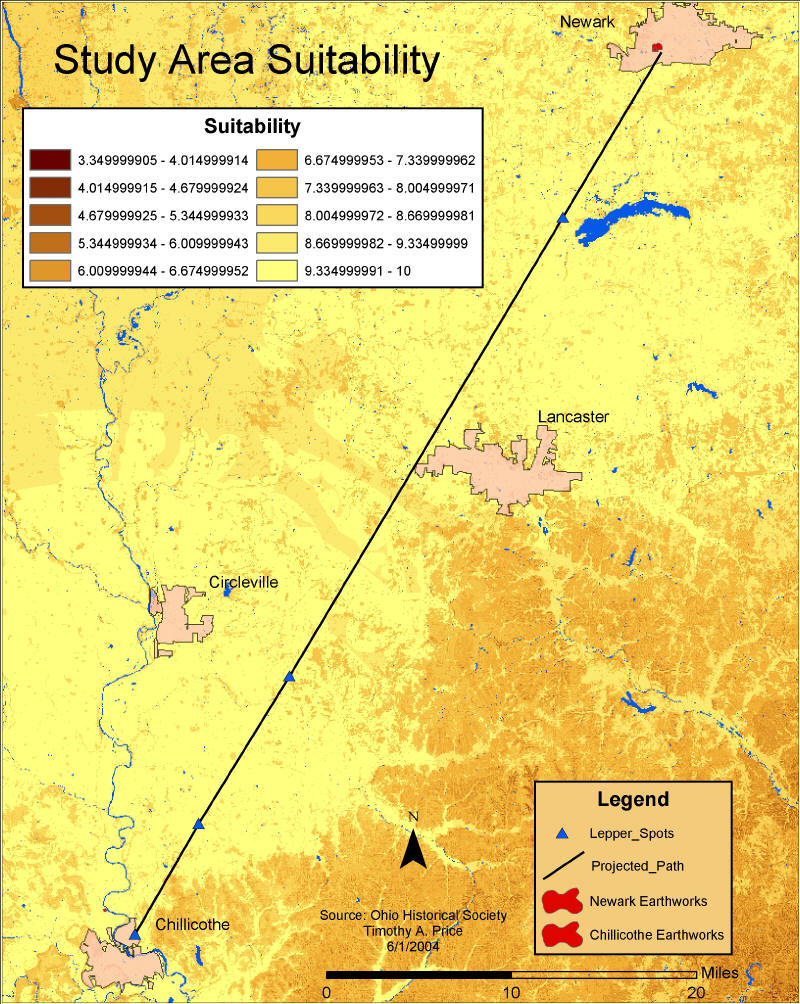
This new raster was saved as “Suitability” (Figure 12) and depicts the areas most likely for a Hopewell road to have been built upon. Suitability is assigned on a scale of 1–10, with 10 being the most likely places where a road might have been built. A cost model was created next so that the shortest route could be identified without all of the variables included in the suitability model. Cost models identify optimum corridors and factor in economic, environmental, or other objectives. For this model, the dataset of the cost of traveling over the landscape was based on the fact that it is more costly to traverse steep slopes and construct a road on certain land types. Locations with low cost values identify the areas that will be the least costly to build a road through. To achieve this portion of the model, the percent slope (percent_slope) and land use grids were once again reclassified. Slope was reclassified (step14_slope) so that steeper slopes were give a higher number (10 = maximum slope). Those with the lowest slope were given a value of 1. Land cover was also reclassified (step14_land) so that the most desirable lands were given a value of 1, next most desirable lands were given a 2, and the third most desirable lands a 3. The two files were combined and weighted as follows:
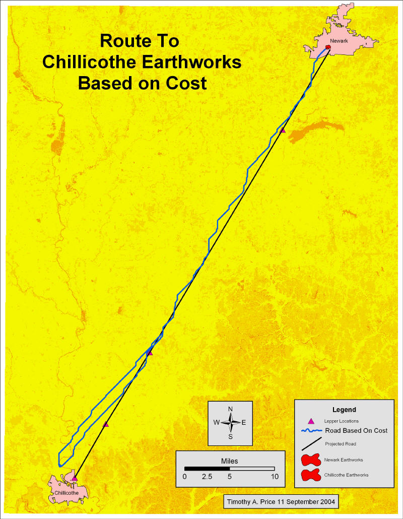
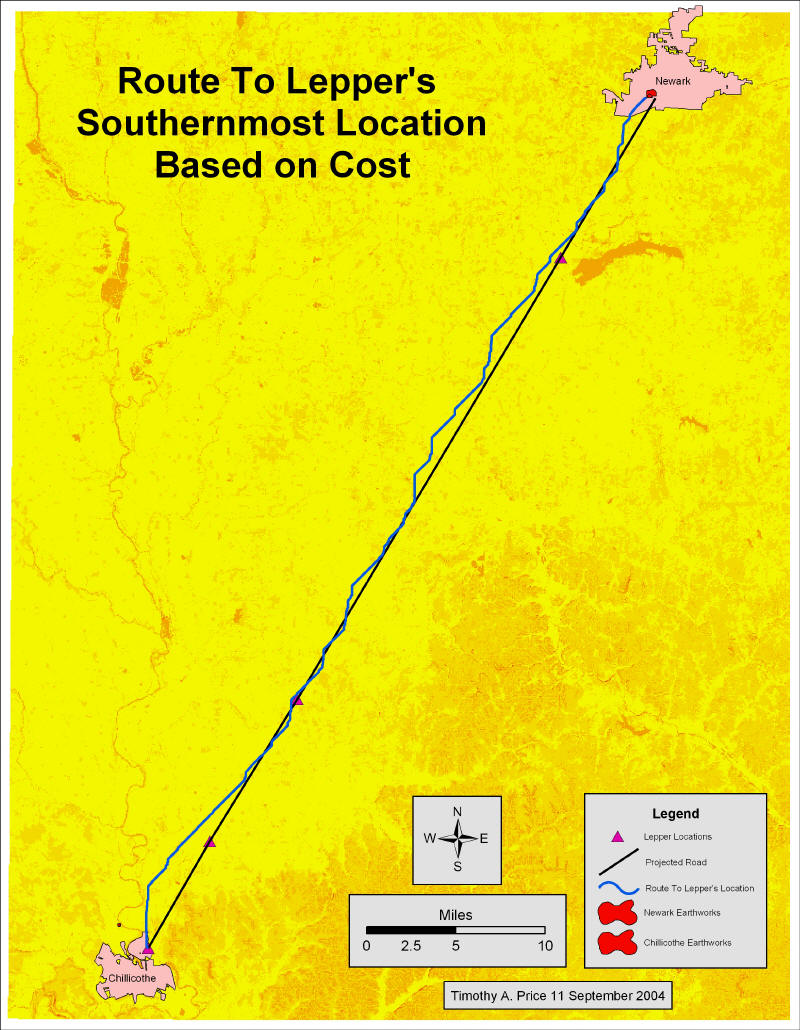
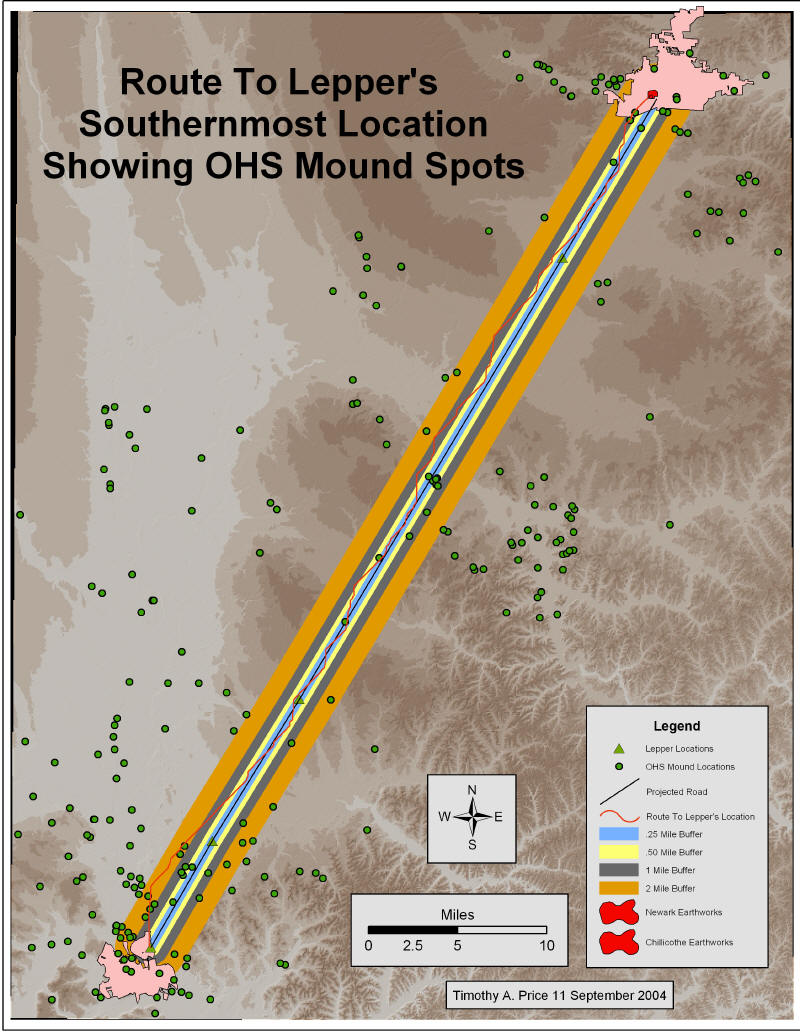
To see if the possibility of a Hopewell Road was more fact than fiction, several cost-weighted distance/shortest distance calculations were performed using the spatial analyst extension of ArcMap. These included the following: a) Distance to the Newark Earthworks using the suitability grid (Suitability) as the cost input raster (cdist2). A direction grid (cdir2) was also created at this time. Next, the shortest distance was calculated to the southernmost Lepper location. In addition to the above calculations, a test was performed on the suitability model. Steps required to produce the original model had their values reversed. For example, the river data file had another straight line distance calculation done. This was then reclassified into equal intervals. Values of 1 were assigned to areas closest to rivers (the most suitable locations), while values of 10 were assigned to areas farthest from rivers (the least suitable locations). Areas in between were ranked. This procedure was done to see if the ranking system itself made any difference in the route of the predicted road based on the numerous factors included in the suitability model. b) Distance to the Newark Earthworks using the cost grid (Cost) as the cost input raster (cdist1). A direction grid (cdir1) was also created at this time. The shortest route was then calculated using the Chillicothe Earthworks as the destination. c) Shortest path was calculated again using the cost layer with the southernmost Lepper location as the destination. Once all of the calculations were completed, maps were produced of the possible routes of the Great Hopewell Road. Chapter 5 Another problem with this type of analysis is that the variables used to determine site locations are based solely upon the physical environment. Commonly used variables for predicting site location include distance to water, slope, and soil drainage. In using variables representing only the physical environment, any qualitative, non-environmentally based decision-making on location preference is precluded. Hence, while the majority of sites may be referenced through this method, special purpose sites, which may not have been selected on the basis of environmental feasibility, would be skipped. John Waldron, 1998 Recent work done by researchers in the Chaco Canyon area of the American Southwest extensively utilized many of the methods discussed in this study (Nials et al 1987). Researchers there relied heavily on the use of aerial photos, both current and archival, and found that they provided the most efficient means of locating prehistoric roads. Additionally, their report notes that archaeological structures – especially small, horseshoe- to circular-shaped structures – were often located along these roadways. There are ample correlations between the proposed Hopewellian road and the Anasazi roads of Chaco Canyon. Circular earthworks are associated with both cultures and may have been located at regular intervals along the “Road to Chillicothe” just as they were along the prehistoric roads of Chaco Canyon. While this study is not able to conclusively determine the existence of a Great Hopewell Road, it does set the stage for further research. In so doing, this study looked at several variables that might have influenced the Hopewell’s way of thinking when it came to deciding on just where to construct a road that stretched for 60 miles or more. This study examined proximity to water bodies, rivers, and other earthworks, as well as slope and land cover. Then, these factors were combined and became the basis for a “suitability” examination of the study area. This was the preliminary step in determining which factors likely were important to the Hopewell in locating their road and which were not. Figure 13 depicts the paths that such a road might have taken had all these factors been important to the Hopewell. Clearly, these potential routes do not follow the projected route between Newark and Chillicothe. This, then, raises the natural question of which variables are essential to our calculations and which are likely extraneous. Next, a model of the route was completed that looked solely at slope and land cover between the earthworks located in Newark and those found in Chillicothe (Figure 14). This possible route follows Lepper’s predicted route extremely closely, deviating most on the southern portion. Moreover, this model shows two possible routes that the Road might have taken in the south. I was unable to ascertain exactly why two routes were drawn in the model, but I do have a theory. Land cover was classified as suitable for the area of the split, and slope at that point is approximately 2.4 percent. Both would have been desirable qualities for the model. The only explanation that justifies this split is the fact that it occurs exactly where the Salt Creek River would cross the route. For the final part of this model, the area between Newark and the southernmost point that Brad Lepper believes to be of the Road was examined. Again using slope and land cover as the main criteria, the shortest path between the two points was determined (Figure 15). In this model, the fit of the route again deviates only in the southern portion of the study area, but alters course to connect with Lepper’s location. It is this model that most closely follows Lepper’s predicted route of the Great Hopewell Road. Indeed, the majority of the model falls within a one-half-mile buffer zone of the projected road, while the entire model falls within two miles. Chapter 6 Accompanying some of the [Ohio] enclosures is another class which has been denominated Graded Ways or Avenues, the purposes of which are not clear… J.P. MacLean, 1879 How has this examination contributed to an understanding of the Hopewellian achievement? In the case of the Great Hopewell Road, the use of GIS has determined that it is likely that a prehistoric connection did indeed exist between Chillicothe and Newark. Indeed, GIS has proven to be an ideal tool as a means to combine information from the past embedded in the landscape to reveal new dimensions of the existing information. While Lepper’s idea of the road’s existence initially brought together a wealth of information, GIS allowed for further extrapolation of the existing data. Moreover, while the evidence discovered in this research is based solely on the use of computer-assisted modeling, it is nonetheless important to furthering the discussion on the existence of a Hopewellian road. Slope and land cover made the most impact on the outcome of this study. It would appear that the physical landscape transpired with land use to reveal an astonishingly accurate connection between the two major archaeological sites located near Newark and Chillicothe, Ohio. Indeed, these considerations, as applied in the various models, appear to support Lepper’s conclusion that the Hopewell “designed and laid out [the road] with great care and with intimate familiarity of the intervening landscape”. The fact that the majority of the model that examined the area between Newark and Lepper’s southernmost point fell within one half mile to one mile of the projected route is extremely significant; indeed, many portions follow the projected route almost exactly. As a byproduct of this research, a second discovery was also reveled that is highly worthy of not only mention, but further investigation. Upon closer examination, the map showing the Ohio Historical Society’s ancient mound locations reveals a significant number of “events” that occur within the projected path’s buffer zones. Fifty four mounds fall within a two-mile buffer; 25 are within one mile, and twelve are within one half of a mile (Figure 16). Looking back at the mound density map, figure 11, it becomes quickly apparent that the Ohio Valley was indeed a hotbed of prehistoric Indian activity. Perhaps the road was a means of connecting these various places, or, more likely, the mounds were part of villages that sprang up along the way as it was being built. With the advances of radio-carbon dating in the field of archaeology, it might be possible to put a chronology to the sites located nearby that may help determine when the road may have been built and, possibly, in which direction the Hopewell might have started from. While the “function of the Great Hopewell Road remains unknown, similar structures built by the Maya were monumental expressions of politico-religious connections between centers” (Schele and Freidel 1990:353). Only further investigations will allow researchers to find clues that may one day unravel these continuing mysteries. Still though, no matter how many aerial photographs are taken, or satellite images analyzed, researchers will not be able to firmly establish the extent of the road until excavations occur proving that these sites are, indeed, earthwork remnants. Unfortunately, excavation requires time, money, and the permission of the people who own the land – something that is not always readily available. Until such time as this occurs, researchers will continue in their quest for knowledge using the best tools available to them – GIS is just such a tool. Chapter 7 Aldenderfer, Mark. 1986. Anthropology, Space, and Geographic Information Systems. Oxford University Press, Oxford, UK. Allen, K.M., S.W. Green, and E.B.W. Zubrow, eds. 1990. Interpreting Space: GIS and Archaeology. Taylor & Francis, London. Atwater, Caleb. 1820. Description of the Antiquities Discovered in the State of Ohio and Other Western States. Archaeologia Americana, vol. 1, pp. 105-267. Aveni, Anthony F. 2000. Between The Lines: The Mystery of the Giant Ground Drawings of Ancient Nasca, Peru. University of Texas Press, Austin, Tex. Corliss, William R. 2000. Science Frontiers Online, Volume 127 Ebert, James I. 2000. See Westcott. Gerber, N’omi B., and Katharine C. Ruhl. 2000. The Hopewell Site: A Contemporary Analysis Based on the Work of Charles C. Willoughby. Eastern National. Kavasch, E. Barrie. 2004. The Mound Builders of Ancient North America. iUniverse, Inc., New York. Lepper, Bradley T. 1994. The Great Hopewell Road: a Middle Woodland Sacra Via Across Central Ohio. Paper presented at the joint meeting of the Midwest Archaeological Conference and the Southeast Archaeological Conference, Lexington, Kentucky. Lepper, Brad T. 1995. Tracing Ohio’s Great Hopewell Road. Archaeology, vol. 45, no. 6, pp. 52 – 56. Lepper, Brad T. 2002. The Newark Earthworks: Monumental Geometry and Astronomy at a Hopewellian Pilgrimage Center. Exhibition catalog, Hero, Hawk, and Open Hand: Ancient Indian Art of the Woodlands, Richard Townsend, ed., The Art Institute of Chicago. MacLean, J.P. 1879. The Mound Builders, Cincinnati, Ohio. American Antiquarian Society Archives, Worcester, Mass. Madry, Scott. n.d. GIS and Remote Sensing for Archaeology: Burgundy, France. Informatics International, Chapel Hill, N.C. Milner, George R. 2004. The Mound Builders: Ancient Peoples of Eastern North America. Thames & Hudson Ltd., London Maschner, Herbert D.G. 1996. New Methods, Old Problems: Geographic Information Systems in Modern Archaeological Research. Center for Archaeological Investigations, Southern Illinois University at Carbondale. Nials, Fred, John Stein, and John Roney. 1987. Chacoan Roads in the Southern Periphery: Results of Phase II of the BLM Chaco Roads Project. Bureau of Land Management, Santa Fe, N. Mex. Pacheco, Paul J., ed. 1998. A View from the Core: A Synthesis of Ohio Hopewell Archaeology. Ohio Archaeological Council, Columbus, Ohio. Putnam, Frederic W. 1888. See Silverberg: 150. Reeves, Dache M. 1936. A Newly Discovered Extension of the Newark Works. Ohio State Archaeological and Historical Quarterly, vol. XLV. Romain, William F. 2000. Mysteries of the Hopewell: Astronomers, Geometers, and Magicians of the Eastern Woodlands. The University of Akron Press, Akron, Ohio. Salisbury, J.A., and C.B. Salisbury. 1862. Accurate Surveys & Descriptions of the Ancient Earthworks at Newark, Ohio. American Antiquarian Society, Worcester, Mass. Schele, L., and D. Freidel. 1990. A Forest of Kings. William Morrow, New York. Sheets, Payson D., and Brian R. McKee. 1994. Archaeology, Volcanism, and Remote Sensing in the Arenal Region, Costa Rica. The University of Texas Press, Austin, Tex. Silverberg, Robert. 1986. The Mound Builders of Ancient America: The Archaeology of a Myth. Abridged version. Ohio University Press, Athens, Ohio. Squier, E.G., and E.H. Davis. 1848. Ancient Monuments of the Mississippi Valley. Smithsonian Contributions to Knowledge, vol. 1, Smithsonian Institution. Trombold, Charles D. 1991. Ancient Road Networks and Settlement Hierarchies in the New World. Cambridge University Press, Cambridge, Great Britain. Waldron, John. 1998. The Delineation and Analysis of Prehistoric Landscape and Culture in Southeast Ohio: A GIS Approach. Ohio University thesis, Athens, Ohio. Westcott, Konnie L., and R. Joe Brandon. 2000. Practical Applications of GIS for Archaeologists: A Predictive Modeling Toolkit. Taylor & Francis, Philadelphia, Pa. Wheatley, David, and Mark Gillings. 2002. Spatial Technology and Archaeology: The archaeological applications of GIS. Taylor & Francis, Philadelphia, Pa. Wyrick, D. 1866. Ancient Works near Newark, Licking County, Ohio. Atlas of Licking County, Ohio, Beers, Soule, & Co., New York |
|||||||||||||||||||||||||||||||||||||||||||||||||||||||||||||||||||||||
|
Timothy-Price.com © 2012 |
